So you're trying to choose an event-study estimator...
event_study.RmdThe command event_study presents a common syntax that
estimates the event-study TWFE model for treatment-effect heterogeneity
robust estimators recommended by the literature and returns all the
estimates in a data.frame for easy plotting by the command
plot_event_study. The general syntax is
event_study(
    data, yname, idname, tname, gname,
    estimator,
    xformla = NULL, horizon = NULL, weights = NULL
)
The option data specifies the data set that contains the
variables for the analysis. The four other required options are all
names of variables: yname corresponds with the outcome
variable of interest; idname is the variable corresponding
to the (unique) unit identifier, \(i\);
tname is the variable corresponding to the time-period,
\(t\); and gname is a
variable indicating the period when treatment first starts
(group-status).
| Estimator | R package and Estimator Option | Type | Comparison group | Main Assumptions | Uniform inference of estimates |
|---|---|---|---|---|---|
Gardner (2021) |
Imputes \(Y(0)\) | Not-yet- and/or Never-treated |
|
||
Borusyak, Jaravel, and Spiess (2021) |
|
Imputes \(Y(0)\) | Not-yet- and/or Never-treated |
|
|
Callaway and Sant'Anna (2021) |
2x2 Aggregation | Either Not-yet- or Never-treated |
|
✔ | |
Sun and Abraham (2020) |
|
2x2 Aggregation | Not-yet- and/or Never-treated |
|
|
Roth and Sant'Anna (2021) |
|
2x2 Aggregation | Not-yet-treated |
|
|
| * Anticipation can be accounted for by adjusting 'initial treatment day' back \(x\) periods, where \(x\) is the number of periods before treatment that anticipation can occur. | |||||
There are five main estimators available and the choice is specified
for the estimator argument and are described in the table
above.1
The following paragraphs will aim to highlight the differences and
commonalities between estimators. These estimators fall into two broad
categories of estimators. First, did2s and
{didimputation} are imputation-based
estimators as described above. Both rely on “residualizing” the outcome
variable \(\tilde{Y} = Y_{it} - \hat{\mu}_g -
\hat{\eta}_t\) and then averaging those \(\tilde{Y}\) to estimate the event-study
average treatment effect \(\tau^k\).
These two estimators return identical point estimates, but differ in
their asymptotic regime and hence their standard errors.
The second type of estimator, which we label 2x2
aggregation, takes a different approach for estimating
event-study average treatment effects. The packages did,
fixest and {staggered} first estimate \(\tau_{gt}\) for all group-time pairs. To
estimate a particular \(\tau_{gt}\),
they use a two-period (periods \(t\)
and \(g-1\)) and two-group (group \(g\) and a “control group”)
difference-in-differences estimator, known as a 2x2
difference-in-differences. The particular “control group” they use will
differ based on estimator and is discussed in the next paragraph. Then,
the estimator manually aggregate \(\tau_{gt}\) across all groups that were
treated for (at least) \(k\) periods to
estimate the event-study average treatment effect \(\tau^k\).
These estimators do not all rely on the same underlying assumptions, so the rest of the table tries to concisely summarize the differences between estimators. The comparison group column describes which units are utilized as comparison groups in the estimator and hence will determine which units need to satisfy a parallel trends assumption. For example, in some circumstances, treated units will look very different from never-treated units. In this case, parallel trends may only hold between ever-treated units and hence only these units should be used in estimation. In other cases, for example if treatment is assigned randomly, then it’s reasonable to assume that both not-yet- and never-treated units would all satisfy parallel trends.
For estimators labeled “Not-yet- and/or never-treated”, the default
is to use both not-yet- and never-treated units in the estimator.
However, if all never-treated units are dropped from the data set before
using the estimator, then these estimators will use only not-yet-treated
groups as the comparison group. did provides an option to
use either the not-yet- treated or the never- treated group as
a comparison group depending on which group a researcher thinks will
make a better comparison group. {staggered} will
automatically drop units that are never treated from the sample and
hence only use not-yet-treated groups as a comparison group.
The next column, Main Assumptions, tries to summarize
concisely the main theoretical assumptions underlying each estimator.
First, the assumptions about parallel trends match the previous
discussion on the correct comparison group. The only estimator that
doesn’t rely on a parallel trends assumption is
{staggered}, instead relying on the assumption that
when a unit receives treatment is random.
The next assumption, that is common across all estimators, is that there should be “limited anticipation” of treatment. In general, anticipatory effects are when units respond to treatment before it is actually implemented. For example, this can be common if the news of a treatment triggers behavior responses before the treatment is put in place. “Limited anticipation” is when these anticipatory effects can only exist in a “few” pre-periods.2 In any of these cases, “treatment” should be manually moved back by the maximum number of periods where anticipation can occur. For example, if treatment starts in 2012 and anticipatory effects are reasonably only possible 2 years before, this units’ “group” should be labelled as 2010 in the data.
The imputation-based estimators require an additional assumption that the parametric model of \(Y(0) = \mu_i + \eta_t + \varepsilon_{it}\) is correctly specified. This is because in the first stage, you have to accurately impute \(Y(0)\) when residualizing \(Y\) which relies on the correct specification of \(Y(0)\). The 2x2 aggregation models does not impute \(Y(0)\) and hence only relies on a parallel trends assumption. The last column highlights that did allows for uniform inference of estimates. This addresses the problem that multiple hypotheses tests are being done by researchers (e.g. checking individually if all post periods significant) by creating standard errors that adjust for multiple testing.
Example usage of event_study
The result of event_study is a tibble in a
tidy format that contains point estimates and standard
errors for each relative time indicator for each individual estimator.
The results of event_study is a dataframe with event-study
term, the estimate, standard error, and a column containing a character
for which estimator is used. This output dataframe will in turn be
passed to plot_event_study for easy comparison. We return
to the df_het dataset to see example usage of these
functions.
library(did2s)
#> Loading required package: fixest
#> did2s (v1.0.0). For more information on the methodology, visit <https://www.kylebutts.github.io/did2s>
#>
#> To cite did2s in publications use:
#>
#>   Butts, Kyle (2021).  did2s: Two-Stage Difference-in-Differences
#>   Following Gardner (2021). R package version 1.0.0.
#>
#> A BibTeX entry for LaTeX users is
#>
#>   @Manual{,
#>     title = {did2s: Two-Stage Difference-in-Differences Following Gardner (2021)},
#>     author = {Kyle Butts},
#>     year = {2021},
#>     url = {https://github.com/kylebutts/did2s/},
#>   }
data(df_het, package = "did2s")
out = event_study(
  data = df_het, yname = "dep_var", idname = "unit",
  tname = "year", gname = "g", estimator = "all"
)
#> Note these estimators rely on different underlying assumptions. See Table 2 of `https://arxiv.org/abs/2109.05913` for an overview.
#> Estimating TWFE Model
#> Estimating using Gardner (2021)
#> Estimating using Callaway and Sant'Anna (2020)
#> Estimating using Sun and Abraham (2020)
#> Estimating using Borusyak, Jaravel, Spiess (2021)
#> Estimating using Roth and Sant'Anna (2021)

head(out)
#>    estimator  term   estimate  std.error
#>       <char> <num>      <num>      <num>
#> 1:      TWFE   -20 0.04097725 0.07167704
#> 2:      TWFE   -19 0.13665695 0.07147683
#> 3:      TWFE   -18 0.14015820 0.07245520
#> 4:      TWFE   -17 0.15793252 0.07431871
#> 5:      TWFE   -16 0.09910002 0.07379570
#> 6:      TWFE   -15 0.20561127 0.07116478
plot_event_study(out, horizon = c(-5,10))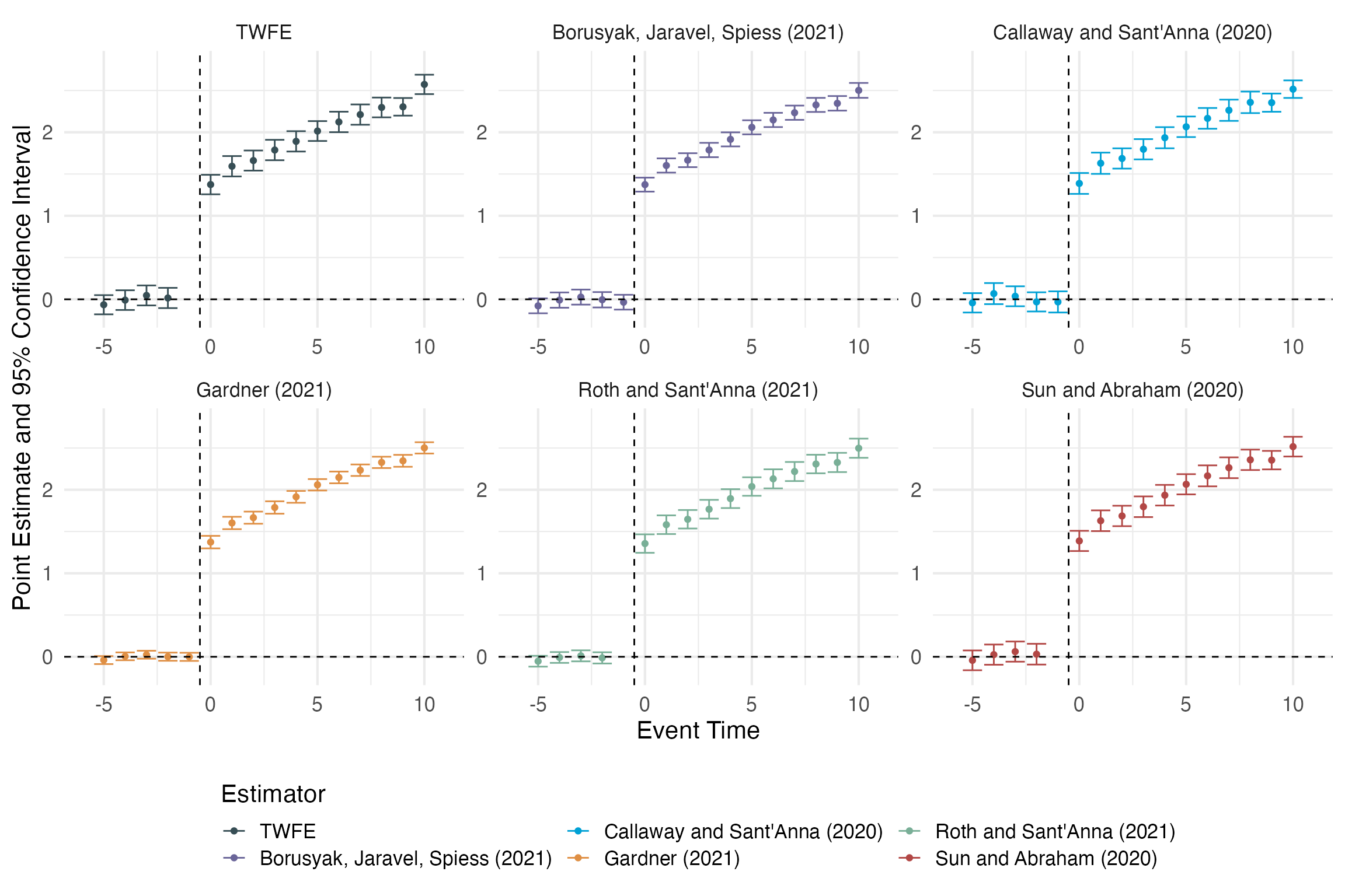
Event-study Estimators