Two-Stage Difference-in-Differences

Two-stage Difference-in-differences, Gardner (2021)

Researchers often want to a difference-in-differences (DiD) model in a regression setting. Typically, these have made use of the so-called twoway fixed effects (TWFE) framework. For example, in a static setting:

\[\begin{equation} y_{it} = \mu_i + \mu_t + \tau D_{it} + \varepsilon_{it}, \end{equation}\]

where \(\mu_i\) are unit fixed effects, \(\mu_t\) are time fixed effects, and \(D_{it}\) is an indicator for receiving treatment.

Similarly, a (dynamic) event-study TWFE model could be written as:

\[\begin{equation} y_{it} = \mu_i + \mu_t + \sum_{k = -L}^{-2} \tau^k D_{it}^k + \sum_{k = 1}^{K} \tau^k D_{it}^k + \varepsilon_{it}, \end{equation}\]

where \(D_{it}^k\) are lag/leads of treatment (k periods from initial treatment date).

Aside: Sometimes researches use variants of this model where they bin or drop leads and lags.

However, running OLS to estimate either model has been shown to not recover an average treatment effect and has the potential to be severely misleading in cases of treatment effect heterogeneity Borusyak et. al. (2021); Callaway and Sant’Anna (2020); de Chaisemartin and d’Haultfoeuille (2020); Goodman-Bacon (2021); Sun and Abraham (2020)].

One way of thinking about this problem is through the Frisch–Waugh–Lovell (FWL) theorem. When estimating the unit and time fixed effects, you create a residualized \(\tilde{Y}_{it}\) which is commonly said to be “the outcome variable after removing time shocks and fixed units characteristics”, but you also create a residulaized \(\tilde{D}_{it}\) or \(\tilde{D}_{it}^k\). To simplify the literature, this residualized treatment indicators is what creates the problem of interpreting \(\tau\) or \(\tau^k\), especially when treatment effects are heterogeneous.

That’s where Gardner (2021) comes in. What Gardner does to fix the problem is quite simple: estimate \(\mu_i\) and \(\mu_t\) seperately so you don’t residualize the treatment indicators. In the absence of treatment, the TWFE model gives you a model for (potentially unobserved) untreated outcomes

\[y_{it}(0) = \mu_i + \mu_t + \varepsilon_{it}.\]

Therefore, if you can consistently estimate \(y_{it}(0)\), you can impute the untreated outcome and remove that from the observed outcome \(y_{it}\). The value of \(y_{it} - \hat{y}_{it}(0)\) should be close to zero for control units and should be close to \(\tau_{it}\) for treated observations. Then, regressing \(y_{it} - \hat{y}_{it}(0)\) on the treatment variables should give unbiased estimates of treatment effects (either static or dynamic/event-study).

Aside: This is the same logic as the new paper by [Borusyak et. al. (2021).

The steps of the two-step estimator are:

1. First estimate \(\mu_i\) and \(\mu_t\) using untreated/not-yet-treated observations, i.e. the subsample with \(D_{it}=0\). Residualize outcomes \(\tilde{y}_{it} = y_{it} - \hat{\mu}_i - \hat{\mu}_t\).

2. Regress \(\tilde{y}_{it}\) on \(D_{it}\) or \(D_{it}^k\)’s to estimate the treatment effect \(\tau\) or \(\tau^k\)’s.

Some notes:

Standard Errors

First, the standard errors on \(\tau\) or \(\tau^k\)’s will be incorrect as the dependent variable is itself an estimate. This is referred to the generated regressor problem in econometrics parlance. Therefore, Gardner (2021) has developed a GMM estimator that will give asymptotically correct standard errors.

Details are left to the paper, but are implemented in this R package

Anticipation

Second, this procedure works so long as \(\mu_i\) and \(\mu_t\) are consistently estimated. The key is to use only untreated/not-yet-treated observations to estimate the fixed effects. For example, if you used observations with \(D_{it} = 1\), you would attribute treatment effects \(\tau\) as “fixed characteristics” and would combine \(\mu_i\) with the treatment effects.

The fixed effects could be biased/inconsistent if there are anticipation effects, i.e. units respond before treatment starts. The fix is fairly simple, simply “shift” treatment date earlier by as many years as you suspect anticipation to occur (e.g. 2 years before treatment starts) and estimate on the subsample where the shifted treatment equals zero.

This R package allows you to specify the variable \(D_{it}\), if you suspect anticipation, provide the shifted variable to this option.

Covariates

This method works with pre-determined covariates as well. Augment the above step 1. to include \(X_i\) and remove that from \(y_{it}\) along with the fixed effects to get \(\tilde{y}_{it}\).

did2s R Package

did2s is an R package that implements the two-stage DiD procedure described above. To install the package, run the following:

remotes::install_github("kylebutts/did2s")

Note: Windows users should install Rtools before running the above command, since they will need to compile some C++ code from source.

The main function is did2s(), which estimates the two-stage DiD procedure. The function is really a convenience wrapper (plus some important transformations) around fixest::feols() and will return a fixest object. This is important for several reasons that will become clear in the examples that follow.

did2s() requires the following arguments:

• yname: The outcome variable. For example, "y".
• first_stage: Formula indicating the first stage. This can include fixed effects and covariates, but do not include treatment variable(s)! For efficiency, it is recommended to use the fixest convention of specifying fixed effects after a vertical bar. For example, ~ x1 + x2 | fe1 + fe2.
• second_stage: Formula indicating the treatment variable or, in the case of event studies, treatment variables. Again, following fixest conventions, it is recommended to use the i() syntax. For example, ~ i(time_to_treatment, ref = 0).
• treatment: A binary (1/0) or logical (TRUE/FALSE) variable demarcating when treatment turns on for a unit. For example, "treated".

Optional arguments include the ability to implement weighted regressions and whether to cluster or bootstrap standard errors.

Example

Let’s walk through an example dataset from the package.

library(did2s) ## The main package. Will automatically load fixest as well.
#> Loading required package: fixest
#> did2s (v1.0.2). For more information on the methodology, visit <https://www.kylebutts.github.io/did2s>
#> 
#> To cite did2s in publications use:
#> 
#>   Butts, Kyle (2021).  did2s: Two-Stage Difference-in-Differences
#>   Following Gardner (2021). R package version 1.0.2.
#> 
#> A BibTeX entry for LaTeX users is
#> 
#>   @Manual{,
#>     title = {did2s: Two-Stage Difference-in-Differences Following Gardner (2021)},
#>     author = {Kyle Butts},
#>     year = {2021},
#>     url = {https://github.com/kylebutts/did2s/},
#>   }
library(ggplot2) 

## Load heterogeneous treatment dataset from the package
data("df_het")
head(df_het)
#>     unit state   group  unit_fe     g  year     year_fe  treat rel_year
#>    <int> <int>  <char>    <num> <num> <int>       <num> <lgcl>    <num>
#> 1:     1    33 Group 2 7.043016  2010  1990  0.06615889  FALSE      -20
#> 2:     1    33 Group 2 7.043016  2010  1991 -0.03098032  FALSE      -19
#> 3:     1    33 Group 2 7.043016  2010  1992 -0.11960742  FALSE      -18
#> 4:     1    33 Group 2 7.043016  2010  1993  0.12632146  FALSE      -17
#> 5:     1    33 Group 2 7.043016  2010  1994 -0.10692055  FALSE      -16
#> 6:     1    33 Group 2 7.043016  2010  1995 -0.27042020  FALSE      -15
#>    rel_year_binned       error    te te_dynamic  dep_var
#>              <num>       <num> <num>      <num>    <num>
#> 1:              -6 -0.08646599     0          0 7.022709
#> 2:              -6  0.76659269     0          0 7.778628
#> 3:              -6  1.51296819     0          0 8.436377
#> 4:              -6  0.02186978     0          0 7.191207
#> 5:              -6 -0.01760317     0          0 6.918492
#> 6:              -6  2.19452731     0          0 8.967123

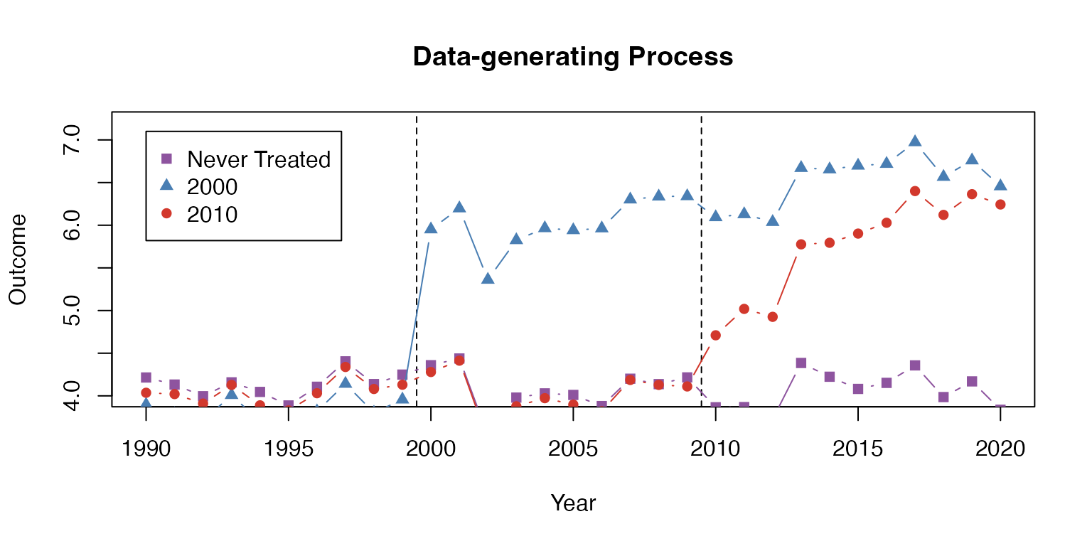
Here is a plot of the average outcome variable for each of the groups:

# Mean for treatment group-year
agg <- aggregate(df_het$dep_var, by=list(g = df_het$g, year = df_het$year), FUN = mean)

agg$g <- as.character(agg$g)
agg$g <- ifelse(agg$g == "0", "Never Treated", agg$g)

never <- agg[agg$g == "Never Treated", ]
g1 <- agg[agg$g == "2000", ]
g2 <- agg[agg$g == "2010", ]


plot(0, 0, xlim = c(1990,2020), ylim = c(4,7.2), type = "n",
     main = "Data-generating Process", ylab = "Outcome", xlab = "Year")
abline(v = c(1999.5, 2009.5), lty = 2)
lines(never$year, never$x, col = "#8e549f", type = "b", pch = 15)
lines(g1$year, g1$x, col = "#497eb3", type = "b", pch = 17)
lines(g2$year, g2$x, col = "#d2382c", type = "b", pch = 16)
legend(x=1990, y=7.1, col = c("#8e549f", "#497eb3", "#d2382c"), 
       pch = c(15, 17, 16),
       legend = c("Never Treated", "2000", "2010"))

Example data with heterogeneous treatment effects

Estimate Two-stage Difference-in-Differences

First, lets estimate a static did. There are two things to note here. First, note that I can use fixest::feols formula including the | for specifying fixed effects and fixest::i for improved factor variable support. Second, note that did2s returns a fixest estimate object, so fixest::esttable, fixest::coefplot, and fixest::iplot all work as expected.

# Static
static <- did2s(df_het, 
                yname = "dep_var", first_stage = ~ 0 | state + year, 
                second_stage = ~i(treat, ref=FALSE), treatment = "treat", 
                cluster_var = "state")
#> Running Two-stage Difference-in-Differences
#>  - first stage formula `~ 0 | state + year`
#>  - second stage formula `~ i(treat, ref = FALSE)`
#>  - The indicator variable that denotes when treatment is on is `treat`
#>  - Standard errors will be clustered by `state`

fixest::esttable(static)
#>                            static
#> Dependent Var.:           dep_var
#>                                  
#> treat = TRUE    2.152*** (0.0476)
#> _______________ _________________
#> S.E. type                  Custom
#> Observations               46,500
#> R2                        0.33790
#> Adj. R2                   0.33790
#> ---
#> Signif. codes: 0 '***' 0.001 '**' 0.01 '*' 0.05 '.' 0.1 ' ' 1

This is very close to the true treatment effect of ~2.23.

Then, let’s estimate an event study did. Note that relative year has a value of Inf for never treated, so I put this as a reference in the second stage formula.

# Event Study
es <- did2s(df_het,
            yname = "dep_var", first_stage = ~ 0 | state + year, 
            second_stage = ~i(rel_year, ref=c(-1, Inf)), treatment = "treat", 
            cluster_var = "state")
#> Running Two-stage Difference-in-Differences
#>  - first stage formula `~ 0 | state + year`
#>  - second stage formula `~ i(rel_year, ref = c(-1, Inf))`
#>  - The indicator variable that denotes when treatment is on is `treat`
#>  - Standard errors will be clustered by `state`

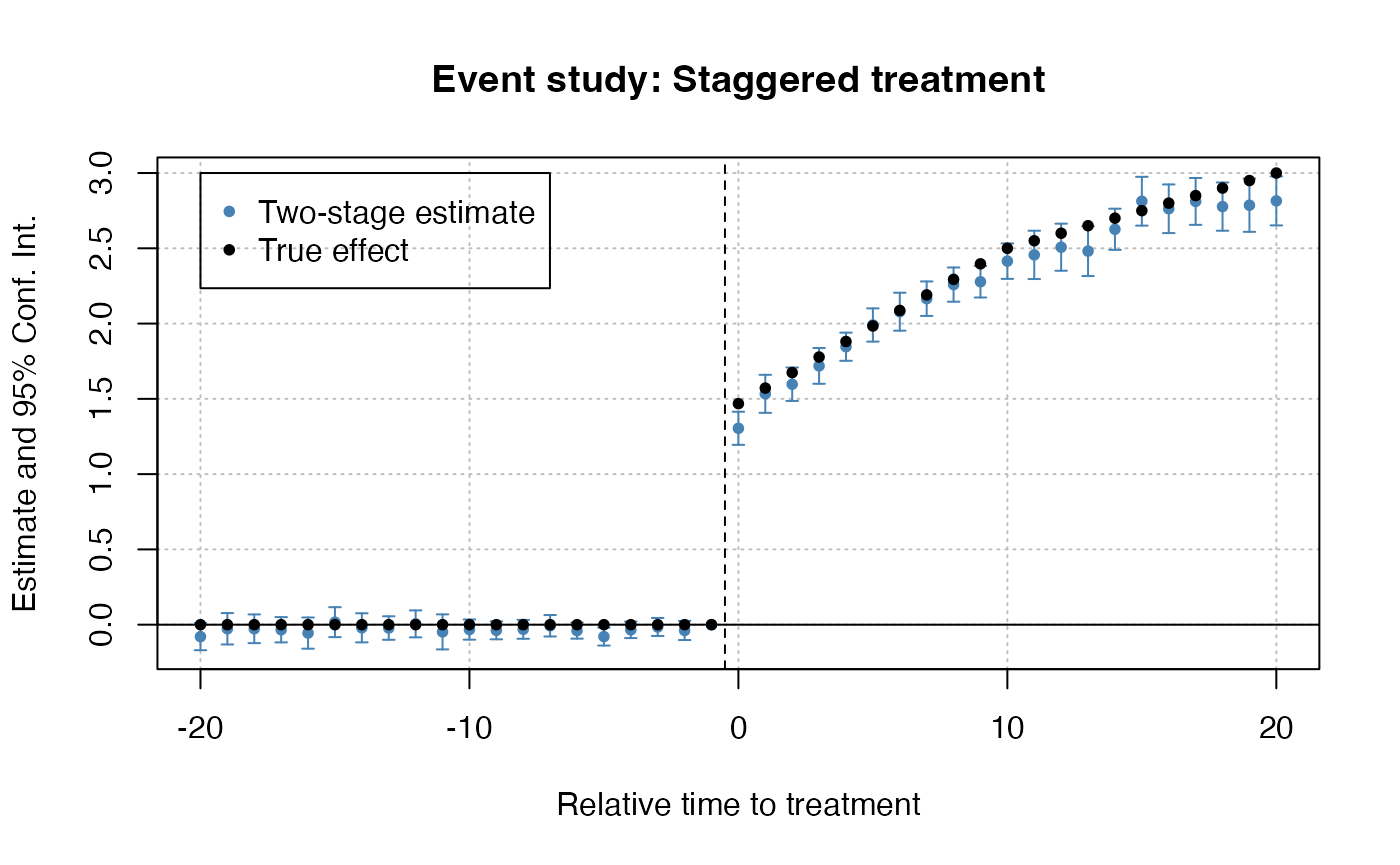
And plot the results:

fixest::iplot(es, main = "Event study: Staggered treatment", xlab = "Relative time to treatment", col = "steelblue", ref.line = -0.5)

# Add the (mean) true effects
true_effects = head(tapply((df_het$te + df_het$te_dynamic), df_het$rel_year, mean), -1)
points(-20:20, true_effects, pch = 20, col = "black")

# Legend
legend(x=-20, y=3, col = c("steelblue", "black"), pch = c(20, 20), 
       legend = c("Two-stage estimate", "True effect"))

Event-study plot with example data

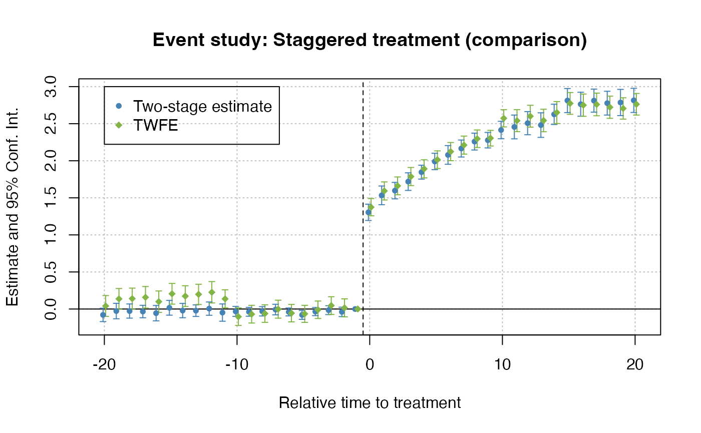
Comparison to TWFE

twfe = feols(dep_var ~ i(rel_year, ref=c(-1, Inf)) | unit + year, data = df_het) 

fixest::iplot(list(es, twfe), sep = 0.2, ref.line = -0.5,
      col = c("steelblue", "#82b446"), pt.pch = c(20, 18), 
      xlab = "Relative time to treatment", 
      main = "Event study: Staggered treatment (comparison)")


# Legend
legend(x=-20, y=3, col = c("steelblue", "#82b446"), pch = c(20, 18), 
       legend = c("Two-stage estimate", "TWFE"))

Citation

If you use this package to produce scientific or commercial publications, please cite according to:

citation(package = "did2s")
#> 
#> To cite did2s in publications use:
#> 
#>   Butts, Kyle (2021).  did2s: Two-Stage Difference-in-Differences
#>   Following Gardner (2021). R package version 1.0.2.
#> 
#> A BibTeX entry for LaTeX users is
#> 
#>   @Manual{,
#>     title = {did2s: Two-Stage Difference-in-Differences Following Gardner (2021)},
#>     author = {Kyle Butts},
#>     year = {2021},
#>     url = {https://github.com/kylebutts/did2s/},
#>   }

References

• Borusyak, Kirill, Xavier Jaravel, and Jann Spiess (2021). “Revisiting Event Study Designs: Robust and Efficient Estimation”, Working Paper.

• Callaway, Brantly, and Pedro H. C. Sant’Anna (2020). “Difference-in-differences with multiple time periods.”, Journal of Econometrics.

• de Chaisemartin, Clement, and Xavier d’Haultfoeuille (2020). “Two-way fixed effects estimators with heterogeneous treatment effects.”, American Economic Review.

• Gardner, John (2021). “Two-Stage Difference-in-Differences.”, Working Paper.

• Goodman-Bacon, Andrew (2021). “Difference-in-differences with variation in treatment timing.”, Journal of Econometrics.

• Sun, Liyang, and Sarah Abraham (2020). “Estimating dynamic treatment effects in event studies with heterogeneous treatment effects.”, Journal of Econometrics.